Single Round Match 790 Editorials - Topcoder

summary: Div2-Easy: Alice’s Birthday For a given , we have to partition the first fibonacci numbers in two set...... #### Div2-Easy: Alice’s Birthday

For a given , we have to partition the first fibonacci numbers in two sets with equal sum. The fact that means that if is a multiple of 3, then I can give to Charlie and to Eric, to Charlie and to Eric, so on and so forth eventually giving to Charlie and to Eric. The other two cases are and .

For the first case, let us try to re-use our previous strategy for the last boxes starting with going to Charlie and to Eric. In the end, we will be left with the first two boxes containing and , respectively. Since, so we can simply give one box to Charlie and other one to Eric.

For the second case, we can try our previous strategy but will always be left with one extra box. The fact that the sum of is odd means that we cannot divide them evenly among Charlie and Eric. Had it been possible to divide it equally, it would mean that the total sum is even, which is not possible and can be proven using induction.

Since we only have to run a loop till , so time complexity is .

Reference sol in Java

import java.io.*; 
import java.util.*; 
import javafx.util.Pair;

public class AlicesBirthday {
    public int[] partition(int k) {
	int[] arr = {-1} ;
	if(k % 3 == 1) return arr ; 
	
        ArrayList<Integer> charlie = new ArrayList<Integer>(), eric = new ArrayList<Integer>(); 
	while(k > 2) {
	    charlie.add(k--);
	    eric.add(k--); eric.add(k--);
	}
	if(k == 2) { 
	    eric.add(k--);
	    charlie.add(k--);
	}
	int[] ret = new int[charlie.size()]; int index = 0;
	for (Integer value: charlie) 
   		ret[index++] = value;
	return ret;
    }
}

Reference sol in Python

class AlicesBirthday:
	def partition(self, K):
		F = [1, 1]
		while len(F) < K: F.append( F[-1] + F[-2] )
		F = F[:K]
		charlie, eric, answer = 0, 0, []
		for k in reversed(range(K)):
			if charlie > eric:
				eric += F[k]
			else:
				charlie += F[k]
				answer.append(k+1)
		if charlie == eric:
			return answer
		return [-1]

Div2-Medium: Bob the Builder

Suppose we are at the given height . At any step, we can either move to one of its factors or add to it. While we can move to its factors without any cost, we have to spend $ to add . So, basically, we have a given state, few possible options from there, and we want to find out end whether a specific end state (i.e. height ) is reachable or not. If reachable, we have to do so in minimum cost. This naturally appeals to be modeled by graphs with states representing the nodes and edges representing the transitions. Thus, we have to find the shortest path in a graph, so Dijkstra definitely comes as the first solution in mind.

One may use Dijkstra to solve the problem, but it is not immediately clear when to stop exploring if there does not exist any path. We would never actually need to go beyond (proof is shown below). But going so high, Dijkstra may get TLE. The fact that edge weights are only and means that we can use instead of Dijkstra and the time limit was high enough to allow that in case exploration goes so high. However, in practice, the max step explored before reaching a goal seems to be quite low (the worst case we could find was not more than ); hence normal Dijkstra passes easily.

Reference sol in Java using 0-1 BFS

import java.util.*;
import java.lang.*;
import java.io.*;

public class BobtheBuilder {
    public int N = (int) 5e5 + 2 ; 
    public int maxStep = -1 ; 
    public List <Integer>[] factors = new ArrayList[N];
    public int dist[] = new int[N] ; 
    public boolean seen[] = new boolean[N] ; 
    
    void prep() {
	    for(int i = 1; i < N; i++) {
	        factors[i] = new ArrayList<Integer> (); 
	        dist[i] = (int) 2e9 ; seen[i] = false ; 
	        int sq = (int) Math.sqrt(i);
	        for(int j = 1; j <= sq; j++) {
	            if(i % j == 0) {
	                factors[i].add(j); factors[i].add(i/j);
	            }
	        }
	    }
    }
    public int minimumPrice(int b, int k, int h) {
	prep();
        Deque<Integer> deq = new ArrayDeque<Integer>(); // seen[b] = true ; 
        dist[b] = 0 ;
        deq.addFirst(b);
        while(deq.size() > 0) {
            int top = deq.removeFirst(); if(top > maxStep) maxStep = top ; 
            if(top == h) return dist[top] ;
            for(int f : factors[top]) {
                if(dist[top] < dist[f]) {
                    deq.addFirst(f);
                    dist[f] = dist[top] ; 
                }
            }
            if( (top + k) < N) {
                if( (dist[top] + 1) < dist[top + k]) {
                    dist[top + k] = dist[top] + 1 ;
                    deq.addLast(top + k); 
                }
            }
        }
        return -1 ; 
    }
}

Reference sol in C++ using Dijkstra

#include <bits/stdc++.h>
using namespace std;

struct record {
    int id;
    int dist;
};

bool operator<(const record &A, const record &B) {
    if (A.dist != B.dist) return A.dist < B.dist;
    return A.id < B.id;
}

int solve(int start, int add, int goal) {
    int div = __gcd(add,goal);
    if (start % div) return -1;

    vector<int> D(1002000,2000000);
    D[start] = 0;
    set<record> Q;
    Q.insert( {start, 0} );
    while (!Q.empty()) {
        record kde = *Q.begin();
        Q.erase( Q.begin() );
        if (kde.id >= 1002000) continue;
        if (kde.id == goal) break;
        for (int div=1; div*div<=kde.id; ++div) if (kde.id % div == 0) {
            vector<int> opts = {div, kde.id/div};
            for (int kam : opts) {
                int ndist = kde.dist;
                if (ndist >= D[kam]) continue;
                Q.erase( {kam, D[kam]} );
                D[kam] = ndist;
                Q.insert( {kam, D[kam]} );
            }
        }
        vector<int> opts = { kde.id + add };
        for (int kam : opts) {
            int ndist = kde.dist + 1;
            if (ndist >= D[kam]) continue;
            Q.erase( {kam, D[kam]} );
            D[kam] = ndist;
            Q.insert( {kam, D[kam]} );
        }
    }
    if (D[goal] == 2000000) return -1;
    return D[goal];
}

struct BobtheBuilder {
    int minimumPrice(int B, int K, int H) { return solve(B,K,H); }
};

Proof
If we are at some state , then at anytime, we can go to one of its factors (possibly itself) or add . We do this starting from until we reach . Suppose it is possible to reach , then thinking about the process in reverse is basically from we can go to one of its multiple (possibly itself) or subtract and continue this loop until we reach . Thus, we can model this in the following form:

Simplifying this, we reduce it to a well-known form:

So, we end up with a linear diophantine equation. Let

. This is only solvable when

so we can instantly return -1 if

is not a multiple of

. The fact that

have opposite signs means that this admits infinite positive solutions. From

Bezuot’s Identity

, we can always find a pair

such that

and

. So we can always find

lie in the range

and since infinite positive solutions are possible and we can shift

, so it’s always possible to find a pair

with both lying in

. Since

, so the max state we need to explore to ensure we always find a solution is bounded by

. Once we reach

from

, we can repeat the same process to reach

from

. While we did the derivation in the reverse form, it obviously holds in the forward manner starting from

. Some useful links:

1. Details on Bezout’s Identity
2. Positive Solution of Linear Diophantine Eq

Div2-Hard / Div1-Easy: The Social Network

We are given an undirected connected graph with exponential weights of the form , and we have to find its minimum cut. The problem may look intimidating but what is in favor for us is the fact that all edge weights are distinct.

Let the given weights sorted in decreasing order be (i.e. edge weight is ). Then, for any valid between and , we have

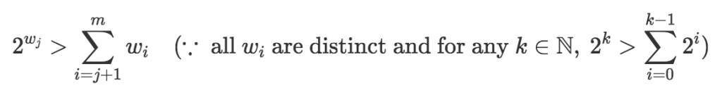
So, we would like to keep the edge with the highest weight out of the cut edges set at the cost of ending up with all other edges in the cut since their total sum is strictly less than the highest weight. Thus, we can keep adding edges one by one in the graph (in decreasing order of their weight) as long as one whole connected component does not form.

The edges which do not get added in the graph form our cut edges, and their sum is the answer. This can be done by DSU but was not required since the constraints were significantly small. If we do use DSU, then sorting dominates the runtime with total complexity as .

Reference Sol in Java

import java.util.*;
import java.lang.*;
import java.io.*;

public class TheSocialNetwork {
    
    class Edge implements Comparable<Edge> {
        public int u;
        public int v;
        public int w;
        
        public Edge(int uu, int vv, int cc) {
            this.u = uu;
            this.v = vv;
            this.w = cc;
        }
        
        public int compareTo(Edge c) {
            if (w < c.w) return 1;
            if (w > c.w) return -1;
            return 0;
        }
    }
        
    int M = 1002 ; int C = 100002 ; int N = 302 ; 
    List <Edge> edges = new ArrayList<Edge>() ; 
    int[] par = new int[N] ; int[] sz = new int[N] ; int[] pwr = new int[C] ; 
    int MOD = (int) (1e9 + 7); int comp ; 
    
    boolean[] seen = new boolean[C] ;
    List < Integer >[] adj = new ArrayList[N] ; 
    boolean[] visited = new boolean[N] ;
    int connected ;
    
    void prepare() {
        pwr[0] = 1 ; seen[0] = false ; 
        for(int i = 1; i < C; i++) {
            pwr[i] = (pwr[i-1] * 2) % MOD ;
            seen[i] = false ;
        }
        for(int i = 1; i < N; i++) {
            par[i] = i ; sz[i] = 1 ;
            adj[i] = new ArrayList<Integer>(); 
            visited[i] = false ;
        }
    }
    
    int getPar(int v) {
        if(par[v] == v) return v ;
        else return par[v] = getPar(par[v]); 
    }
    
    int dsu(int u, int v) {
        int parU = getPar(u) ; int parV = getPar(v);
        if(parU == parV) return 0;
        
        if(sz[u] < sz[v]) { // swap
            u ^= v ; v ^= u ; u ^= v ; 
        }
        sz[u] += sz[v] ;
        par[parV] = parU ; 
        return 1 ;
    }
    
    public int minimumCut(int n, int m, int[] u, int[] v, int[] l) {
        prepare();
        for(int i = 0; i < m; i++) {
            Edge e = new Edge(u[i], v[i], l[i]);
            edges.add(e); 
        }
        Collections.sort(edges);
        int ans = 0; comp = n ; 
        for(Edge e : edges) {
            System.out.println(e.w);
            int parU = getPar(e.u) ; int parV = getPar(e.v);
            if(parU == parV) {
            }
            else {
                if(comp > 2) { 
                    comp-- ;
                    dsu(e.u, e.v);
                }
                else {
                    ans += pwr[e.w] ; 
                    ans %= MOD ; 
                }
            }
        }
        return ans ; 
    }    
}

Reference Sol in Python

def pow2(n):
	if n == 0: return 1
	t = pow2(n//2)
	t *= t
	if n % 2: t *= 2
	return t % 1000000007

class TheSocialNetwork:
	def minimumCut(self, n, m, u, v, l):
		edges = [ (-z,x-1,y-1) for x,y,z in zip(u,v,l) ]
                edges.sort()
                component_count = n
                component = list(range(n))
		answer = 0
		for w,x,y in edges:
			if component[x] == component[y]: continue
			if component_count == 2:
				answer = (answer + pow2(-w)) % 1000000007
			else:
				cx, cy = component[x], component[y]
				component = [ cx if c==cy else c for c in component ]
				component_count -= 1
		return answer

Side Thought: We were wondering whether it is possible to solve this problem using max-flow?

Div1-Medium: Proposal Optimization

Such kind of ratio problems can be solved by using a niche trick. I think it is hard to develop this line of thinking unless you have encountered it before.

Let us say the optimal ratio is . Thus, . What we can do is a binary search on , and check if a ratio is feasible or not. So, for a given , we have to check whether is possible, which is the same thing as (let’s call the L.H.S. ). The constraints on seem to be quite high to do any form of DP while constraints on the grid’s dimension, are quite low although obviously not permitting brute force solutions. However, meet-in-the-middle looks promising since we can store while doing brute force from one corner of the grid and checking from another (meeting in cells lying on some sort of diagonal of the grid).

In fact, it is the intended solution, and we also have to take care of the costs along with to actually know if any of the options is actually feasible. So, when doing brute from one side, we store pairs on those diagonal cells and later sort them according to to ease our process in the next brute. While doing brute from the other end, we have , and we want the highest whose cost satisfies . By storing in prefix maximum manner, we can binary search on the highest index option with cost and take its (since we already sorted) to get our answer.

The best diagonal cells for a grid of size would be the set . Since x, so the number of such diagonal cells (let us denote that by ) can’t exceed . We can focus on the analysis of square matrix since it will dominate the rectangular grids. Let the number of binary search iterations required to find the optimal ratio be (80 iterations suffice for error). To reach a diagonal cell there are ways and then we have to binary search on those many paths which we got from first brute force. Thus, doing meet-in-the-middle takes

Hence, the total time required is bounded by

.

Reference Sol in C++

#include <bits/stdc++.h>
#include<ext/pb_ds/assoc_container.hpp>
#include<ext/pb_ds/tree_policy.hpp>

using namespace std ;
using namespace __gnu_pbds;

template <typename T> // *s.find_by_order(0), s.order_of_key(2) ;
using ordered_set = tree<T, null_type, less<T>, rb_tree_tag, tree_order_statistics_node_update>;

#define reMin(a, b) a = min(a, b)
#define reMax(a, b) a = max(a, b)

#define lint long long
#define pb push_back
#define F first 
#define S second 
#define sz(x) (int)x.size()
#define all(x) begin(x), end(x)
#define SET(x, val) memset(x, val, sizeof(x))
#define fastio ios_base::sync_with_stdio(0); cin.tie(0); cout.tie(0)

typedef vector < int > vi ;
typedef pair < int, int > pii ;

const int N = 300 + 2 ;
const int MOD = 1e9 + 7 ;
const lint INF = 1e18 ;

double best = 0 ;
int n, m, k ;
int roses[N][N], tulips[N][N], cost[N][N] ;

vector < pair < int, double > > meet[N][N] ;
vector < double > ratios[N][N] ; 
int diagonal ;
bool possible = 0 ;
bool ratioSatisfied = 0 ; 

void down(int i, int j, int rose, int tulip, int totalCost, double& R) {
	if(i >= n or j >= m) return ;
	rose += roses[i][j] ; tulip += tulips[i][j] ; totalCost += cost[i][j] ; 
	if(totalCost > k) return ; 
	if(i + j == diagonal) {
		double cur = rose ; cur -= R * tulip ; 
		meet[i][j].pb({totalCost, cur});
		return ; 
	}
	down(i+1, j, rose, tulip, totalCost, R); down(i, j+1, rose, tulip, totalCost, R); 
}

void up(int i, int j, int rose, int tulip, int totalCost, double& R) {
	if(i < 0 or j < 0) return ;
	rose += roses[i][j] ; tulip += tulips[i][j] ; totalCost += cost[i][j] ; 
	if(totalCost > k) return ; 
	if(i + j == diagonal) {
		rose -= roses[i][j] ; tulip -= tulips[i][j] ; totalCost -= cost[i][j] ; 
		double cur = rose ; cur -= R * tulip ; 

		pair < int, double > item = {k - totalCost, 2e9} ;
		int idx = upper_bound(all(meet[i][j]), item) - meet[i][j].begin();
		idx-- ;
		if(idx >= 0) {
			possible = 1 ; assert(idx < sz(ratios[i][j]) and sz(ratios[i][j]) == sz(meet[i][j]));
			double mx = ratios[i][j][idx] ; 
			
			if((mx + cur) >= 0) // should be EPS!! 
				ratioSatisfied = 1 ; 
		}
		return ; 
	}
	up(i-1, j, rose, tulip, totalCost, R); up(i, j-1, rose, tulip, totalCost, R); 
}

void check(double ratio) {
	down(0, 0, 0, 0, 0, ratio);

	for(int i = 0; i < n; i++) {
		int j = diagonal - i ;
		if(j >= m or j < 0) continue ; 
		
        if(sz(meet[i][j]) <= 0) continue ; 
		sort(all(meet[i][j]));

		ratios[i][j].pb(meet[i][j][0].S);
		for(int p = 1; p < sz(meet[i][j]); p++)
			ratios[i][j].pb(max(meet[i][j][p].S, ratios[i][j].back()));
	}
	up(n-1, m-1, 0, 0, 0, ratio);
}

double solve() {
	double low = 0, high = 1e6 ; ratioSatisfied = 0 ;
	
	for(int iter = 0; iter < 70; iter++) {
		double mid = (low + high) / 2 ;
		check(mid); 
		if(ratioSatisfied) low = mid ;
		else high = mid ;
		
		// clear stuff
		ratioSatisfied = 0 ; 
		for(int i = 0; i < n; i++) {
			int j = diagonal - i ;
			if(j < 0 or j >= m) continue ; 
			ratios[i][j].clear(); meet[i][j].clear();
		}
	}
	return low ; 
}

class ProposalOptimization {
public:
	double bestPath(int rows, int cols, int K, vi roz,  vi tolip, vi expense);
};

double ProposalOptimization::bestPath(int rows, int cols, int K, vi roz,  vi tolip, vi expense ){
	n = rows ; m = cols ; k = K ;
	for(int i = 0; i < n; i++) for(int j = 0; j < m; j++) roses[i][j] = roz[i*cols + j] ; 
	for(int i = 0; i < n; i++) for(int j = 0; j < m; j++) tulips[i][j] = tolip[i* cols + j] ; 
	for(int i = 0; i < n; i++) for(int j = 0; j < m; j++) cost[i][j] = expense[i*cols + j] ; 
	double best = solve();
	if(!possible) return -1 ;
	else return best ; 
}

Reference Sol in Java

import java.util.*;
import java.math.*;
 
public class ProposalOptimization {
    class Option implements Comparable<Option> {
        public int orchids;
        public int tulips;
        public int cost;
 
        public Option(int orchids, int tulips, int cost) {
            this.orchids = orchids;
            this.tulips = tulips;
            this.cost = cost;
        }
 
        public int compareTo(Option c) {
            if (cost < c.cost) return -1;
            if (cost > c.cost) return 1;
            if (orchids < c.orchids) return -1;
            if (orchids > c.orchids) return 1;
            if (tulips < c.tulips) return -1;
            if (tulips > c.tulips) return 1;
            return 0;
        }
    }
 
    Option[][] getOptions(int[][] orchids, int[][] tulips, int[][] costs, int steps, boolean secondPass) {
        int R = orchids.length, C = orchids[0].length;
        int[][] options = new int[][] { {0,0,0,0,0} };
        for (int d=1; d<=steps; ++d) {
            int newOptionCount = 0;
            for (int i=0; i<options.length; ++i) {
                if (options[i][0] + 1 < R) ++newOptionCount;
                if (options[i][1] + 1 < C) ++newOptionCount;
            }
            int[][] newOptions = new int[newOptionCount][5];
            for (int i=0, j=0; i<options.length; ++i) {
                if (options[i][0] + 1 < R) {
                    int r = newOptions[j][0] = options[i][0] + 1;
                    int c = newOptions[j][1] = options[i][1];
                    int mul = (secondPass && d == steps) ? 0 : 1;
                    newOptions[j][2] = options[i][2] + mul * orchids[r][c];
                    newOptions[j][3] = options[i][3] + mul * tulips[r][c];
                    newOptions[j][4] = options[i][4] + mul * costs[r][c];
                    ++j;
                }
                if (options[i][1] + 1 < C) {
                    int r = newOptions[j][0] = options[i][0];
                    int c = newOptions[j][1] = options[i][1] + 1;
                    int mul = (secondPass && d == steps) ? 0 : 1;
                    newOptions[j][2] = options[i][2] + mul * orchids[r][c];
                    newOptions[j][3] = options[i][3] + mul * tulips[r][c];
                    newOptions[j][4] = options[i][4] + mul * costs[r][c];
                    ++j;
                }
            }
            options = newOptions;
        }
        int[] answerCounts = new int[R];
        for (int i=0; i<options.length; ++i) ++answerCounts[options[i][0]];
        Option[][] answer = new Option[R][];
        for (int r=0; r<R; ++r) answer[secondPass ? R-1-r : r] = new Option[answerCounts[r]];
        for (int i=0; i<options.length; ++i) {
            int r = options[i][0];
            answer[secondPass ? R-1-r : r][ --answerCounts[r] ] = new Option( options[i][2], options[i][3], options[i][4] );
            // System.out.println("row "+r+" added option "+options[i][2]+" "+options[i][3]+" "+options[i][4] );
        }
        return answer;
    }
 
    int[][] flip(int[][] array) {
        int R = array.length, C = array[0].length;
        int[][] answer = new int[R][C];
        for (int r=0; r<R; ++r) for (int c=0; c<C; ++c) answer[r][c] = array[R-1-r][C-1-c];
        return answer;
    }
 
    boolean solvable(double x, Option[] options1, Option[] options2, int K) {
        int b = 0;
        double bestb = -1e20;
        for (int a=options1.length-1; a>=0; --a) {
            while (b < options2.length && options1[a].cost + options2[b].cost <= K) {
                bestb = Math.max( bestb, options2[b].orchids - x * options2[b].tulips );
                ++b;
            }
            if (options1[a].orchids - x * options1[a].tulips + bestb >= 0) return true;
        }
        return false;
    }
 
    public double bestPath(int R, int C, int K, int[] _orchids, int[] _tulips, int[] _costs) {
 
        int[][] orchids = new int[R][C];
        int[][] tulips = new int[R][C];
        int[][] costs = new int[R][C];
        for (int r=0; r<R; ++r) for (int c=0; c<C; ++c) {
            orchids[r][c] = _orchids[r*C + c];
            tulips[r][c] = _tulips[r*C + c];
            costs[r][c] = _costs[r*C + c];
        }
 
        Option[][] options1 = getOptions( orchids, tulips, costs, (R+C-2)/2, false);
        Option[][] options2 = getOptions( flip(orchids), flip(tulips), flip(costs), (R+C-1)/2, true);
 
        for (int i=0; i<options1.length; ++i) Arrays.sort(options1[i]);
        for (int i=0; i<options2.length; ++i) Arrays.sort(options2[i]);
 
        int bestCost = K+1;
        for (int i=0; i<options1.length; ++i) if (options1[i].length > 0 && options2[i].length > 0) bestCost = Math.min( bestCost, options1[i][0].cost + options2[i][0].cost );
        if (bestCost > K) return -1;
 
        double lo = 0, hi = 1e6 + 1;
        for (int step=0; step<200; ++step) {
            double med = (lo+hi) / 2;
            boolean isSolvable = false;
            for (int i=0; i<options1.length; ++i) if (solvable(med,options1[i],options2[i],K)) {
                isSolvable = true;
                break;
            }
            if (isSolvable) lo = med; else hi = med;
        }
        return lo;
    }
}

Div1-Hard: Tale Of Two Squares:

#div1 A number can be expressed as a sum of two sqaures if and only if all its prime factors of the form occur even times. So while taking the product of few numbers, we are only interested in its prime decomposition; hence, we can store a bit-vector for each \(A_{i}\) denoting odd/even occurrence of such prime factors.

From now on, **whenever I talk about primes it is assumed to be of the form \(4K+3\) (for some \(k \in Z\) ) and that the reader is familar with basis of a vector space and gaussian elimination. Please go through this if you are not familiar with the usage of those concepts in CP:
Introductory Blog on using Linear Algebraic techniques to solve XOR related problems

Now, \(A_{i}≤10^7\) so # primes is around \(3∗10^5\). Normal Gaussian elimination would easily TLE, even with bitsets. Still, lets imagine doing Gaussian elimination traversing from the highest bit to the lowest and xoring when necessary. Notice that, when you are traversing, if any prime factor \(>\sqrt{ A_{i} }\) exists (at max one can exist), the moment you xor it, no more bits \(>\sqrt{ A_{i} }\) will be on anymore (since only one such was on earlier and now you have xored it). Now, you can simply simulate Gaussian elimination on lower-order primes (i.e. primes\(≤\sqrt{ A_{i} }\)) and handle that one highest bit (if it exists) separately. This way, combined with bitset for lower-order primes, solves the problem without queries.

For queries, let us process them offline. Let \(queries[l]\) store all the queries with their left endpoint as \(l\). We will insert \(A_{i}\) into our basis from the right side, \(i\) going from \(N−1\) to \(0\). After we have inserted the element at index \(i\), we will answer all the queries which begin their, i.e., the ones in \(queries[i]\).

We will use a simple fact about linear combination of vectors but in a clever manner to answer the queries. Suppose we are about to try and insert v into our \(Basis\) (may not insert if it turns out to be dependant). If \(v=b _{1}+b _{2}+⋯b_{k} (where b_{i}∈Basis)\), then we can remove one of the \(b_i\) and instead insert \(v\) into its place, keeping the basis intact. So, we will use this fact while inserting — we will try to keep such elements in the basis which have leftmost index so as to answer as many queries as possible. We can do this greedily: while inserting \(v\), whenever we are about to xor it with some \(b_i\), we will first check which has the least index and \(swap (b_i, v)\) if \(v\) ‘s index is smaller than \(b_i\). If we do end up swapping, then \(v\) becomes a part of the basis (in place of \(b_i\)), and we progress doing Gaussian Elimination with \(b_i\) instead. Otherwise, we move forward with v like we normally do. Please refer to the attached code for more details.

Now, when we answer queries which have left index \(i\), we will have the basis vectors from \(A[i: N]\) having the least possible index. So for a query \(i\) \(R\), we simply need to count how many vectors in our basis have index \(≤R\). This can be easily done with some BIT or set.

Let \(K\) denote the number of primes \(\leq \sqrt{ A_{i} }\)\((=225)\). We store a bitset of size \(K\) for every prime. While doing Gaussian elimination, we handle the large bit manually while following the normal procedure for lower-order primes; hence it takes \(O (\frac{K^2}{64})\) time to insert a \(A_i\). After that, we answer queries at index i in \(O (log (N))\) time by querying in our BIT. Hence, the overall complexity is \(O \left( N⋅ \frac{k^2}{64}+Q⋅log (N) \right)\), dominated by Gaussian elimination using bitsets:

一个数字可以被表示为两个平方数的和，当且仅当它所有形式为 \(4K+3\) 的质因数出现偶数次。所以，当我们计算几个数字的乘积时，我们只关心它的质因数分解；因此，我们可以为每个 \(A_{i}\) 存储一个位向量，表示这些质因数的奇数/偶数出现。

从现在开始，每当我谈到质数时，假定它们为形式为 \(4K+3\)（对于某个 \(k \in Z\)），并且读者熟悉向量空间的基础和高斯消元。如果您对在竞赛编程中如何应用这些概念不熟悉，请阅读这篇文章：使用线性代数技术解决异或相关问题的入门博客

现在，\(A_{i}≤10^7\)，因此质数的数量大约为 \(3∗10^5\)。普通的高斯消元甚至使用位集合也可能很容易超时。不过，让我们假设从最高位到最低位进行高斯消元并在必要时进行异或操作。注意，当您遍历时，如果存在任何大于 \(\sqrt{ A_{i} }\) 的质因数（最多可以存在一个），一旦异或了它，就不会再有大于 \(\sqrt{ A_{i} }\) 的位了（因为之前只有一个位是打开的，现在您已经异或了它）。现在，您可以简单地模拟对低阶质数（即质数 \(≤\sqrt{ A_{i} }\)）进行高斯消元，并单独处理那个最高位（如果存在的话）。这样，结合对低阶质数的位集合处理，就可以解决问题。

对于查询，让我们离线处理它们。让 \(queries[l]\) 存储所有左端点为 \(l\) 的查询。我们将从右侧将 \(A_{i}\) 插入到我们的基向量中，其中 \(i\) 从 \(N-1\) 到 \(0\)。在我们插入索引 \(i\) 处的元素之后，我们将回答所有在那里开始的查询，即 \(queries[i]\) 中的查询。

我们将使用一个关于向量的线性组合的简单事实，但以聪明的方式来回答这些查询。假设我们将要尝试插入 \(v\) 到我们的 \(Basis\)（如果结果是依赖的话，可能不会插入）。如果 \(v=b_{1}+b_{2}+\dots+b_{k}\)（其中 \(b_{i}∈Basis\)），那么我们可以删除 \(b_i\) 中的一个，并将 \(v\) 放在它的位置，保持基向量不变。因此，我们在插入时将使用这一事实。我们将尝试保留基向量中左端的索引，以回答尽可能多的查询。我们可以贪婪地实现这一点：在插入 \(v\) 时，每当我们要与一些 \(b_i\) 进行异或操作时，我们将首先检查哪个索引最小，如果 \(v\) 的索引小于 \(b_i\)，我们将 \(swap(b_i, v)\)。如果最终进行了交换，那么 \(v\) 将成为基向量的一部分（代替 \(b_i\)），并且我们将使用 \(b_i\) 进行高斯消元。否则，我们将像正常情况一样继续进行。更多细节，请参考附加的代码。

现在，当我们回答左端点为 \(i\) 的查询时，我们将拥有基向量 \(A[i:N]\)，其具有可能的最小索引。因此，对于一个查询 \(i\) 到 \(R\)，我们只需要计算基向量中索引 \(≤R\) 的数量。这可以很容易地使用一些 BIT 或 set 完成。

让 \(K\) 表示 \(\leq \sqrt{ A_{i} }\) 的质数的数量（\(=225\)）。我们为每个质数存储一个大小为 \(K\) 的 [[../ACM/bitset]] 。在进行高斯消元时，我们手动处理大位数，然后按照常规程序处理低阶质数；因此，插入 \(A_i\) 花费 \(O (\frac{K^2}{64})\) 的时间。之后，在 \(O (log (N))\) 的时间内回答 \(O (log (N))\) 中的查询。因此，总体复杂度是 \(O \left( N⋅ \frac{k^2}{64}+Q⋅log (N) \right)\)，由使用 [[../ACM/bitset]] 的高斯消元支配。

Reference sol in C++

#include <bits/stdc++.h>
using namespace std;

const int SQRTMAX = 3162;
const int SMALL_PRIME_COUNT = 225;
const int SMALL_PRIMES[] = {3, 7, 11, 19, 23, 31, 43, 47, 59, 67, 71, 79, 83, 103, 107, 127, 131, 139, 151, 163, 167, 179, 191, 199, 211, 223, 227, 239, 251, 263, 271, 283, 307, 311, 331, 347, 359, 367, 379, 383, 419, 431, 439, 443, 463, 467, 479, 487, 491, 499, 503, 523, 547, 563, 571, 587, 599, 607, 619, 631, 643, 647, 659, 683, 691, 719, 727, 739, 743, 751, 787, 811, 823, 827, 839, 859, 863, 883, 887, 907, 911, 919, 947, 967, 971, 983, 991, 1019, 1031, 1039, 1051, 1063, 1087, 1091, 1103, 1123, 1151, 1163, 1171, 1187, 1223, 1231, 1259, 1279, 1283, 1291, 1303, 1307, 1319, 1327, 1367, 1399, 1423, 1427, 1439, 1447, 1451, 1459, 1471, 1483, 1487, 1499, 1511, 1523, 1531, 1543, 1559, 1567, 1571, 1579, 1583, 1607, 1619, 1627, 1663, 1667, 1699, 1723, 1747, 1759, 1783, 1787, 1811, 1823, 1831, 1847, 1867, 1871, 1879, 1907, 1931, 1951, 1979, 1987, 1999, 2003, 2011, 2027, 2039, 2063, 2083, 2087, 2099, 2111, 2131, 2143, 2179, 2203, 2207, 2239, 2243, 2251, 2267, 2287, 2311, 2339, 2347, 2351, 2371, 2383, 2399, 2411, 2423, 2447, 2459, 2467, 2503, 2531, 2539, 2543, 2551, 2579, 2591, 2647, 2659, 2663, 2671, 2683, 2687, 2699, 2707, 2711, 2719, 2731, 2767, 2791, 2803, 2819, 2843, 2851, 2879, 2887, 2903, 2927, 2939, 2963, 2971, 2999, 3011, 3019, 3023, 3067, 3079, 3083, 3119 };
vector<int> SMALL_PRIME_ID, pow2;

struct Fenwick1D { // {{{
    int size;
    vector<int> T;

    Fenwick1D(int maxval) {
        size = 1;
        while (size < maxval) size <<= 1;
        T.clear();
        T.resize(size+1,0);
    }

    void update(int x, int delta) { // assumes 1 <= x <= init_maxval
        while (x <= size) { T[x] += delta; x += x & -x; }
    }

    int sum(int x1, int x2) { // sum in the closed interval [x1,x2]
        int res=0;
        --x1;
        while (x2) { res += T[x2]; x2 -= x2 & -x2; }
        while (x1) { res -= T[x1]; x1 -= x1 & -x1; }
        return res;
    }

    int find(int sum) { // largest z such that sum( [1,z] ) <= sum
        int idx = 0, bitMask = size;
        while (bitMask && (idx < size)) {
            int tIdx = idx + bitMask;
            if (sum >= T[tIdx]) { idx=tIdx; sum -= T[tIdx]; }
            bitMask >>= 1;
        }
        return idx;
    }
}; // }}}

void init() {
    SMALL_PRIME_ID.clear();
    SMALL_PRIME_ID.resize(SQRTMAX+1, -1);
    for (int i=0; i<SMALL_PRIME_COUNT; ++i) SMALL_PRIME_ID[ SMALL_PRIMES[i] ] = i;
    pow2.clear();
    pow2.push_back(1);
    for (int i=1; i<100005; ++i) pow2.push_back( (pow2.back()*2) % 998244353 );
}

struct signature {
    bitset< SMALL_PRIME_COUNT > small_bits;
    int large_bit;
    signature() : large_bit(-1) {}

    int highest_prime() {
        if (large_bit != -1) return large_bit;
        for (int i=SMALL_PRIME_COUNT-1; i>=0; --i) if (small_bits.test(i)) return SMALL_PRIMES[i];
        return 0;
    }

    void do_xor(const signature &other) {
        if (other.large_bit != -1) {
            if (large_bit != -1) {
                assert( large_bit == other.large_bit );
                large_bit = -1;
            } else {
                large_bit = other.large_bit;
            }
        }
        small_bits ^= other.small_bits;
    }
};

ostream& operator<< (ostream& out, const signature &S) {
    /*
    int max = SMALL_PRIME_COUNT - 1;
    while (max > 0 && !S.small_bits.test(max)) --max;
    for (int i=0; i<=max; ++i) out << int( S.small_bits.test(i) );
    */
    if (S.large_bit != -1) out << S.large_bit << "+";
    for (int i=9; i>=0; --i) out << int(S.small_bits.test(i));
    return out;
}

struct query {
    int l, r;
};

bool operator< (const query &A, const query &B) {
    if (A.l != B.l) return A.l > B.l;
    return A.r < B.r;
}

signature get_signature(int N) {
    signature answer;
    for (int d=2; d*d<=N; ++d) {
        if (N % d) continue;
        int cnt = 0;
        while (N % d == 0) { ++cnt; N /= d; }
        if (d % 4 != 3) continue;
        if (cnt % 2 == 0) continue;
        answer.small_bits.set( SMALL_PRIME_ID[d] );
    }
    if (N > 1 && N % 4 == 3) {
        if (N > SQRTMAX) answer.large_bit = N; else answer.small_bits.set( SMALL_PRIME_ID[N] );
    }
    return answer;
}

struct TaleOfTwoSquares {
    int count(int N, vector<int> Aprefix, int Q, vector<int> Lprefix, vector<int> Rprefix, int seed) {
        init();

        long long state = seed;

        vector<int> A = Aprefix;
        while (int(A.size()) < N) {
            state = (state * 1103515245 + 12345) % (1LL << 31);
            A.push_back(1 + (state % 10000000));
        }

        if (N <= 20) for (int n=0; n<N; ++n) cout << A[n] << ", "; cout << endl;

        vector<int> L = Lprefix, R = Rprefix;
        while (int(L.size()) < Q) {
            state = (state * 1103515245 + 12345) % (1LL << 31);
            int x = state % N;
            state = (state * 1103515245 + 12345) % (1LL << 31);
            int y = state % N;
            L.push_back( min(x,y) );
            R.push_back( max(x,y) );
        }

        if (Q <= 20) for (int n=0; n<Q; ++n) cout << L[n] << ", "; cout << endl;
        if (Q <= 20) for (int n=0; n<Q; ++n) cout << R[n] << ", "; cout << endl;

        vector<signature> B;
        for (int n=0; n<N; ++n) B.push_back( get_signature(A[n]) );

        vector< vector<int> > query_by_L(N);
        for (int q=0; q<Q; ++q) query_by_L[ L[q] ].push_back( R[q] );

        Fenwick1D InBase(N+2);
        int answer = 0;
        unordered_map<int,int> base_by_highest_prime;

        for (int n=N-1; n>=0; --n) {
            // two dummy updates
            InBase.update(N+1,+1);
            InBase.update(N+1,-1);
            // add number A[n] to the base
            if (B[n].highest_prime() != 0) {
                InBase.update(n+1,+1);
                int where = n;
                while (true) {
                    int p = B[where].highest_prime();
                    if (p == 0) {
                        InBase.update(where+1,-1);
                        break;
                    }
                    if (!base_by_highest_prime.count(p)) {
                        base_by_highest_prime[p] = where;
                        break;
                    }
                    int nxt = base_by_highest_prime[p];
                    if (nxt > where) {
                        base_by_highest_prime[p] = where;
                        B[nxt].do_xor( B[where] );
                        where = nxt;
                    } else {
                        B[where].do_xor( B[nxt] );
                    }
                }
            }
            // answer queries that begin here
            for (int r : query_by_L[n]) {
                int length = r-n+1;
                int base_size = InBase.sum(n+1,r+1);
                answer += pow2[length-base_size] - 1;
                answer %= 998244353;
            }
        }

        return answer;
    }
};